PAView

PAView works to establish links to educators throughout the Commonwealth to develop partnerships, create training opportunities, and provide training and informational materials to support education in remote sensing. These efforts include supporting the annual PA DCNR Remote Sensing Workshop and developing lessongs and tutorials. Some PAView related efforts are included in this section of the site.
Frazier School District Half Earth Lesson
Through this lesson, students will be introduced to the Half-Earth Project by E.O. Wilson. Using the data from www.half-earth.org, students will explore conservancy and preservation projects around the world, designed to preserve half of the land and oceans. According to Wilson, if we can preserve half of the Earth, we can potentially save up to 85% of the world's species can be saved from extinction. See the Story Map: https://storymaps.arcgis.com/stories/abda661068c1490b875bb1e488033c1c
Pennsylvania Western University (formerly Clarion University) and WisconsinView
California University of Pennsylvania, teachers, and WisconsinView created a lesson on Wildfires, Remote Sensing and Emergency Response with a goal of being able to see the future of fires using satellites. In addition, Clarion University provided raster analyses for the project.
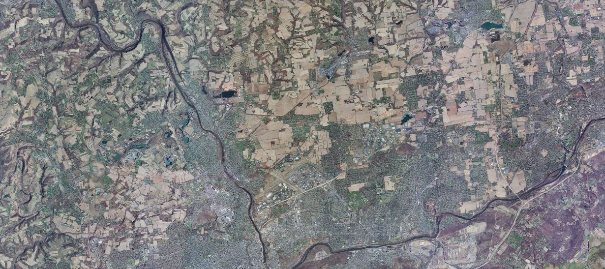
In the state of Pennsylvania, Allegheny County has the second largest population after Philadelphia. For some time, the county’s population has witnessed a steady and continuous decline. Not until the last 10 years that its population started to show some increase. According to the latest Census data of 2020, Allegheny County witnessed a 2.2% increase from 2010. Moon Township was one of the largest communities that had a significant population increase during this period (12.6%). On the other hand, Marshall Township, located in the north and shares a border with Butler county’s Cranberry township, has almost doubled its population (45.8%) during the same period. In this study, we take a deeper look at the spatial changes that occurred during the last 10 years. Assessment of vegetation cover in general and tree cover in specific was conducted. However, despite the significant population growth of those areas, the results show a general increase in vegetation cover in both townships. The methods used in the current study adopted modified vegetation indices that were calculated from high resolution multispectral aerial images, as well as the extraction of tree cover from LiDAR point cloud data. The results show potentials and challenges of those methods. Finally, it is suggested that more structured accuracy assessment to be conducted on the presented results, and method refinements to include other hybrid techniques are to be investigated.
Transport of sediment through small streams is linked to agricultural soil loss, erosion and deposition in stream channels, and ultimately to the sediment that is choking parts of the Chesapeake Bay. Earlier research at Bucknell developed GIS (Geographic Information Systems) tools to calculate, based on a high-resolution digital elevation model (DEM), a sediment transport capacity index, Tc for any point along a stream or concentrated flow path. It is defined as the product of the land area contributing runoff at a point and the slope of the channel at that point (Moore and Wilson, 1992). Earlier work showed a significant correlation between Tc at a point along a flow path and another variable dependent only on DEM data. That other variable is based on the difference between the land surface elevations measured by LIDAR in 2006 and in 2017 (Edif), where positive values indicate erosion and negative values indicate deposition. In a channel transporting large amounts of sediment, erosion and deposition likely occur repeatedly over storms, seasons, and years, with some parts of a reach showing deposition and others erosion. A strong case can be made that high variability in Edif within a reach corresponds to large flows of sediment in the reach, and high sediment flow should correspond to high Tc values. Specifically, the earlier work showed that the standard deviation of Edif, that is, std(Edif), is significantly and positively correlated with Tc. Figure 1 describes how the Edif layer can inform the evolution of the thalweg (the path of the deepest part of the channel).
Marine debris (MD) is a major threat to ecosystems, biodiversity, and human health because it is prevalent in the environment, resistant to degradation, and easily transported for long distance dispersal. MD includes any human-made items that are intentionally or unintentionally discarded in the ocean, including plastics, metals, glass, fishing gear, lumber, etc. In the tropics, hurricanes and other tropical storms are anecdotally considered sources of MD, but their impact is difficult to assess. Combining remote sensing imagery before and after a hurricane with on-the-ground collections of marine debris in the impacted coastal area will greatly improve our understanding of tropical storms as accumulators and depositors of MD along the coast. On 18 September 2022 at 2:00 pm local time, Hurricane Fiona had reached a wind speed of 75 knots and was passing the coastal area of southwest Puerto Rico adjacent to Playa Ballena, a beach that accumulates large quantities of MD throughout the year.
Bucknell Sediment Transport Assessment
Geographic Information Systems (GIS) can use high-resolution Lidar and multispectral images collected from aircraft to provide detailed maps of various characteristics of a watershed. In tributaries to the Chesapeake Bay, including the Susquehanna River, sediment transport is of particular interest because of its impact on the Chesapeake ecosystem. Sediment may originate in tiny rills in the upland areas of a watershed, or in the main channel as bank erosion. This work focuses on mechanisms that work at a scale in between the rill and the channel network scale. Previous work at Bucknell has concentrated on flow path modeling and using digital elevation models (DEMs) along with Land Use and Land Cover (LULC) maps to develop an index of pollution potential in concentrated runoff flow paths. Last summer (2019) a new index was developed, based on work by Moore and Wilson (1992). This work used the stream power index (representing flow rate multiplied by slope) to represent the capacity of a flow path to carry sediment. Based on the assumption that high sediment transport capacity corresponds with high sediment transport during large floods, maps showing sediment transport capacity along concentrated flow paths were developed. Data to evaluate various indices were not available in 2019 because of dry weather during the weeks available for research. In 2020, plans were made to measure sediment deposition in upland areas, but COVID-19 restrictions made collection of these data impossible this summer. The work this summer attempted to validate various sediment transport indices by using two high resolution DEMs taken 11 years apart (in 2006 and 2017). Actual differences (presumably not numerical artifacts) between these two DEMs should represent soil erosion or deposition. Figure 1 is a topographic map of the watershed. Figure 2 is a map showing the difference in elevations between these two DEMs at a 1 m horizontal scale. Light colors represent erosion and dark colors represent deposition
Marine debris (MD) is a major threat to ecosystems, biodiversity, and human health because it is prevalent in the environment, resistant to degradation, and easily transported for long distance dispersal. MD includes any human-made items that are intentionally or unintentionally discarded in the ocean, including plastics, metals, glass, fishing gear, lumber, etc. In the tropics, hurricanes and other tropical storms are anecdotally considered sources of MD, but their impact is difficult to assess. Combining remote sensing imagery before and after a hurricane with on-the-ground collections of marine debris in the impacted coastal area will greatly improve our understanding of tropical storms as accumulators and depositors of MD along the coast. On 18 September 2022 at 2:00 pm local time, Hurricane Fiona had reached a wind speed of 75 knots and was passing the coastal area of southwest Puerto Rico adjacent to Playa Ballena, a beach that accumulates large quantities of MD throughout the year.
Precision Conservation Mapping on Turtle Creek Watershed in Union County, PA
Watershed managers with limited resources need methods to prioritize possible restoration or remediation sites. The Chesapeake Conservancy developed a Geographical Information System (GIS) – based method to assist in this prioritization. Their method involved use of land-use / land_cover (LULC) maps and high-resolution digital elevation models (DEMs), and resulted in maps of concentrated flow paths, color-coded according to the value of an index called NDFI, representing the likelihood of a path carrying high concentrations of pollutants. Work in this area at Bucknell started in the 2014-15 academic year with a series of consultations with staff from Chesapeake Conservancy to better understand their methodology. The work continued in the 2015-16 academic year when maps of NDFI for Buffalo Creek were developed. Over the course of academic years 2016-17 and 2017-18 work was focused on the development of an Overland Flow Sediment Index (OFSI), tailored for sediment as the pollutant of interest. During the summer of 2019, Bucknell researchers worked with an alternative, physically-based index for sediment transport in watersheds.
Cropland and ArcGIS Online Exercise: Pixels and Crop Changes
This exercise developed by Dr. Tom Mueller of California University of Pennsylvania addresses two National Geographic Standards:
The objective of this exercise is to help students analyze raster data to examine spatial patterns.
Examining Cropscape and the Changes to Agriculture in PA
In introducing students to GIS technologies, PaView partner California University of Pennsyvlania created a lesson for college freshmen or high school seniors. This lesson, which takes approximately two class sessions reinforces the National Geographic Standards: Standard 1: How to use maps and other geographic representations, geospatial technologies, and spatial thinking to understand and communicate information Standard 14: How human actions modify the physical environment Objectives. After this assignment, students should be able to: - Explain raster data and its complexities - Analyze raster data to examine spatial patterns.
In 2020, Villanova purchased Pleiades and WorldView-2 (WV-2) satellite imagery of the area of the marshes of Plum Island Sound, Massachusetts (Figure 1) with the Pennsylvania View (PA View) grant funding. The imagery acquired with grant funding was in June of 2017 and June of 2018 for NDVI analysis, and was augmented with a supplemental department purchase of WorldView-3 (WV-3) satellite imagery from January 2018 to perform ice raft analysis. The WV3 imagery acquired would be just after the January 2018 Northeastern U.S. blizzard (bomb cyclone) and the June imagery from 2017 and 2018 were used to perform vegetation analysis to determine the extent of winter storm damage on the marsh habitat. The Plum Island marshes are a study area for one of the Villanova Environmental Science graduate students who is investigating the effect of storms on sediment deposition including via a mechanism called ice rafting.
Assessment of the Land Classification System Used for Property Valuation in Clarion County
Land classification is directly linked with property valuation. In Clarion County, the currently used land classification is outdated, not only in terms of age (1958) but also in terms of processing and integration within the valuation procedures. This project will evaluate the current state of data as well as processes for land valuation in Clarion County, and, using remotely sensed data and GIS techniques, new estimates for land classification will be produced and tested. The produced system will be also compared with the current one. Change estimates will be produced in order to evaluate the transformation in the quality of land during the past 50 years.
ArcGIS Online Shark Migration Tutorial
The Marine Conservation Science Institute, known for its Expedition WhiteShark shared their great white locational data with PAVIew. Megan Boger, a California University of Pennsylvania student, and Dr. Mueller created an ArcGIS lesson using the data.
Using ARCGIS Online to Create a Map for Recreational Boating
Overview - This tutorial, created by Tim Linkenheimer of the Blackhawk Middle and High School, familiarizes users with the following ArcGIS Online commands and functions: with using the following commands offered in ArcGIS online: Utilizing all of the standard functions such as search, zoom, print, save, share, print and bookmark; Using the Basemap command to load a topographic map provided by ESRI; Using spreadsheet software to load a series of points of reference on a map that are important to locate while traveling; Editing those points of interest so they are categorized, easy to interpret and represented properly on the map.
Plate Tectonics Activity using ArcGIS data
Overview – This activity, created by Lee Cristofano of Bethel Park High School, consists of students, working alone or in small groups, plotting the locations of earthquakes and volcanoes on a map of the Earth. By doing this, the “big idea” of this lesson is for students to discover the correlation between earthquake and volcano locations and the boundaries of the Earth’s tectonic plates. Further, this is evidence that the plates are actually in motion. This lesson is recommended for Grades 7-9 in an Earth and Space Science class.
An Analysis of Earthquakes and Volcanoes Using ArcGIS Online
This online, GIS –based activity allows students to use inquiry-based science to draw conclusions about the relationship between volcanic activity, fault lines and plate tectonics. They will use ArcGIS online mapping tools to arrive at their conclusions. A working ArcGIS mapping account is required for this activity. Ideally, this lesson would be taught after a lesson that introduces ArcGIS mapmaker and would be used as a method to scaffold learning from prior knowledge. The estimated time for this activity is between 60 and 90 minutes, depending on the skill level of the students. Beginner skills in ArcGIS are necessary.Author: Karen Babyak Scully, Southeastern Greene School District
PaView is an AmericaView partner.